Detection of light sources from environment maps
This article presents a Python implementation of an algorithm for detecting light sources from environment maps, LDR or HDR, that uses a equirectangular projection.
However, it can also be used with simple background images or cubemaps with some minor modifications.
Some of the uses cases of such an algorithm can be: raytracing applications where you want to detect the primary light sources for which to issue rays, even in rasterized renderers it can be used to cast shadows that use the environment map, but can also be used in highlight removal applications such as AR.
The algorithm involves the following steps:
There are many algorithms for image downscaling, bilinear filtering is the fastest and easiest to implement which should work best in most cases.
For luminance conversion the standard formula can be used for both LDR and HDR images:
lum = img[:, :, 0] * 0.2126 + img[:, :, 1] * 0.7152 + img[:, :, 2] * 0.0722
Optionally, you can apply a small blur on the luminance image, such as 1-2px for a 1024 image resolution, to remove any high-frequency details (like the image downscaling).
The most common used projection for environment maps is equirectangular projection3, the algorithm will work with other projections such as: panoramic and cube maps, however only equirectangular will be covered here.
First, the image coordinates need to be normalized:
pos[0] = x / width
pos[1] = y / height
Then we need to convert from and to cartesian coordinates by using spherical coordinates, i.e. θ and φ, where θ = x * 2π and φ = y * π.
def sphereToEquirectangular(pos):
  invAngles = (0.1591, 0.3183)
  xy = (math.atan2(pos[1], pos[0]), math.asin(pos[2]))
  xy = (xy[0] * invAngles[0], xy[1] * invAngles[1])
  return (xy[0] + 0.5, xy[1] + 0.5)

def equirectangularToSphere(pos):
  angles = (1 / 0.1591, 1 / 0.3183)
  thetaPhi = (pos[0] - 0.5, pos[1] - 0.5)
  thetaPhi = (thetaPhi[0] * angles[0], thetaPhi[1] * angles[1])

  length = math.cos(thetaPhi[1])
  return (math.cos(thetaPhi[0]) * length, math.sin(thetaPhi[0]) * length, math.sin(thetaPhi[1]))
The next step is to apply a quasi Monte Carlo methond such as Hammersley sampling2 on a sphere:
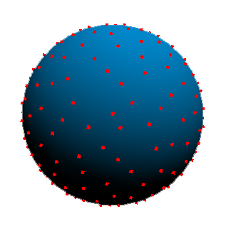
Other sampling methods can be used such as Halton4, however Hammersley is faster and offers a good distribution of the samples on the sphere, Halton is a good choice for plane samples if a simple image is used instead of an environment map.
A requisite for Hammersley sampling is the Van der Corput radical inverse, for more details see references2, a fast implementation of it is:
def vdcSequence(bits):
    bits = (bits << 16) | (bits >> 16)
    bits = ((bits & 0x55555555) << 1) | ((bits & 0xAAAAAAAA) >> 1)
    bits = ((bits & 0x33333333) << 2) | ((bits & 0xCCCCCCCC) >> 2)
    bits = ((bits & 0x0F0F0F0F) << 4) | ((bits & 0xF0F0F0F0) >> 4)
    bits = ((bits & 0x00FF00FF) << 8) | ((bits & 0xFF00FF00) >> 8)
    return float(bits) * 2.3283064365386963e-10 # / 0x100000000

def hammersleySequence(i, N):
    return (float(i) / float(N), vdcSequence(i))
We then use uniform mapping on a sphere:
def sphereSample(u, v):
  PI = 3.14159265358979
  phi = v * 2.0 * PI
  cosTheta = 2.0 * u - 1.0 # map to -1,1
  sinTheta = math.sqrt(1.0 - cosTheta * cosTheta);
  return (math.cos(phi) * sinTheta, math.sin(phi) * sinTheta, cosTheta)
For the Hammersley sampling, we apply a fixed number of samples that is based on the image resolution, we convert from sphere coordinates to cartesian and finally to equirectangular coordinates:
  samplesMultiplier = 0.006
  samples = int(samplesMultiplier * width * height)

  samplesList = []
  # apply hammersley sampling
  for i in range(0, samples):
    xi = hammersleySequence(i, samples)
    xyz = sphereSample(xi[0], xi[1]) # to cartesian
    imagePos = sphereToEquirectangular(xyz)

    luminance = lum[imagePos[0] * width, imagePos[1] * height]
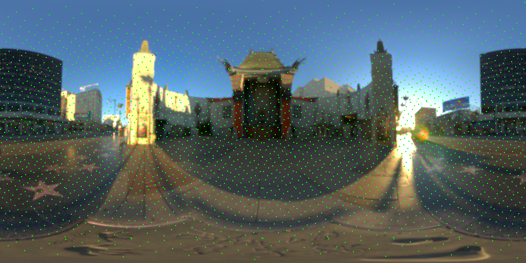
This will give a good distribution of samples that will be checked for light sources:
The first filtering pass will ignore any samples that don't exceed a luminance threshold, this can be higher for HDR maps, afterwards it will sort all samples based on their luminance:
  localSize = int(float(12) * (width / 1024.0)) + 1

  samplesList = []
  # apply hammersley sampling
  for i in range(0, samples):
    xi = hammersleySequence(i, samples)
    xyz = sphereSample(xi[0], xi[1]) # to cartesian
    imagePos = sphereToEquirectangular(xyz)

    luminance = lum[imagePos [0] * width, imagePos [1] * height]
    sample = Sample(luminance, imagePos , xyz)

    luminanceThreshold = 0.8
    #do a neighbour search for the maximum luminance
    nLum = computeNeighborLuminance(lum, width, height, sample.imagePos, localSize)
    if nLum > luminanceThreshold:
      samplesList.append(sample)

  samplesList = sorted(samplesList, key=lambda obj: obj.luminance, reverse=True)
The next pass will filter out based on the Euclidean distance and a pixel distance threshold (which is dependent on the image resolution), a spatial data structure can be used to get rid of the O(N2) complexity:
  euclideanThreshold = int(float(euclideanThresholdPixel) * (width / 2048.0))

  # filter based euclidian distance
  filteredCount = len(samplesList)
  localIndices = np.empty(filteredCount); localIndices.fill(-1)
  for i in range(0, filteredCount):
    cpos = samplesList[i].pos
    if localIndices[i] == -1:
      localIndices[i] = i

      for j in range(0, filteredCount):
        if i != j and localIndices[j] == -1 and distance2d(cpos, samplesList[j].pos) < euclideanThreshold:
          localIndices[j] = i
The resulting samples will go through the merging phase to reduce the number of light sources further:
The final step involves merging the samples that are part of the same light cluster, for this we can use the Bresenham line algorithm and start with the samples with the highest luminance as they were already ordered, when we find a light that passes the Bresenham check we use it's position to adjust the position based on a running weight:
  # apply bresenham check and compute position of the light clusters
  lights = []
  finalIndices = np.empty(filteredCount); finalIndices.fill(-1)
  for i in localIndices:
    sample = samplesList[i]
    startPos = sample.pos
    if finalIndices[i] == -1:
      finalIndices[i] = i

      light = Light()
      light.originalPos = np.array(sample.pos)  # position of the local maxima
      light.worldPos = np.array(sample.worldPos)
      light.pos = np.array(sample.pos)
      light.luminance = sample.luminance

      for j in localIndices:
        if i != j and finalIndices[j] == -1:
          endPos = samplesList[j].pos

          if bresenhamCheck(lum, width, height, startPos[0], startPos[1], endPos[0], endPos[1]):
            finalIndices[j] = i

            # compute final position of the light source
            sampleWeight = samplesList[j].luminance / sample.luminance
            light.pos = light.pos + np.array(endPos) * sampleWeight
            light.pos = light.pos / (1.0 + sampleWeight)

      imagePos = light.pos * np.array([1.0 / width, 1.0 / height)
      light.worldPos = equirectangularToSphere(imagePos)

      lights.append(light)
The Bresenham function involves checking if we have a continous line that has a similar luminance, if the delta at the current pixel exceeds a specific threshold then the check will fail:
def bresenhamCheck(lum, imageSize, x0, y0, x1, y1):

  dX = int(x1 - x0)
  stepX = int((dX > 0) - (dX < 0))
  dX = abs(dX) << 1

  dY = int(y1 - y0)
  stepY = int((dY > 0) - (dY < 0))
  dY = abs(dY) << 1

  luminanceThreshold = 0.15
  prevLum = lum[x0][y0]
  sumLum = 0.0
  c = 0
  if (dX >= dY):
      # delta may go below zero
      delta = int (dY - (dX >> 1))

      while (x0 != x1):
          # reduce delta, while taking into account the corner case of delta == 0
          if ((delta > 0) or (delta == 0 and (stepX > 0))):
              delta -= dX
              y0 += stepY

          delta += dY
          x0 += stepX
          sumLum = sumLum + min(lum[x0][y0], 1.25)
          c = c + 1
          if(abs(sumLum / c - prevLum) > luminanceThreshold and (sumLum / c) < 1.0):
            return 0
  else:
      # delta may go below zero
      delta = int(dX - (dY >> 1))

      while (y0 != y1):
          # reduce delta, while taking into account the corner case of delta == 0
          if ((delta > 0) or (delta == 0 and (stepY > 0))):
              delta -= dY
              x0 += stepX

          delta += dX
          y0 += stepY
          sumLum = sumLum + min(lum[x0][y0], 1.25)
          c = c + 1
          if(abs(sumLum / c - prevLum) > luminanceThreshold and (sumLum / c) < 1.0):
            return 0

  return 1
Note that if needed, further improvements can be done to the Bresenham check which can result in a better merging of the samples, one is to take into account horizontal warping to merge lights which are at the edges, it's also easy to extend it to aproximate the area of the lights sources. Another is to add a distance threshold so you don't merge samples which are too far away.
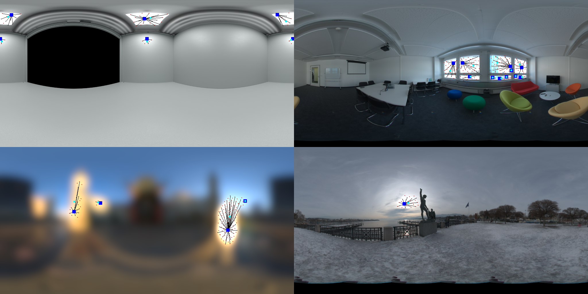
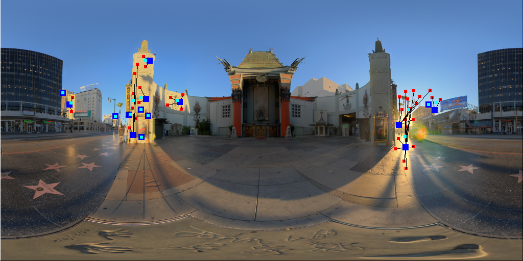
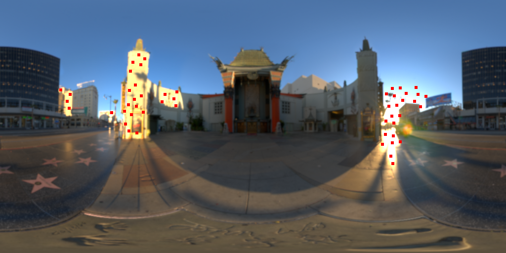
The final results:
Where blue are the local maxima of the light clusters, cyan are the final positions of the light sources, red are samples that are part of the same light cluster with their links.
More results: